This is a project from CS598 Languages and Abstractions for High-Performance Scientific Computing course, which should involve perhaps a week’s worth of focused work (stretched over a long period of course), and it should have a clear end goal, so that it is possible to evaluate at the end whether the stated goals were achieved. This does not mean that you need to get the results you expect (or “good” results, whatever that means), it just means you have to have done a competent job answering your stated question.
⚡ Project proposal
I am going to write an FFT calculation library, targeting CPU and CUDA, aiming to achieve performance comparable to heavily optimized libraries such as FFTW and VkFFT.
I will start from a naive implementation and gradually speed up the program in multiple ways (e.g., single-thread CPU → multi-thread CPU → GPU → better algorithms, kernel fusion, memory coalescing, etc.), showing the speed-up ratio compared to the naive version. For each step, I will use profiling to decide what to improve next.
The possible outcome would be a library that provides performance similar to current FFT libraries such as VkFFT.
Working Progress
Read the SPIRAL paper — understand how it decomposes an FFT calculation. (0.5d)
✅ Done. Since I am limiting the scope to FFT only, DSP components are likely not needed (and difficult to implement).Read the VkFFT paper — understand the reasons for choosing algorithms for parallelizing FFT calculations. (0.5d)
- The most common algorithm is Cooley–Tukey.
- Stockham is commonly used in GPU FFT libraries due to its better cache locality at each step.
- The four-step FFT is used when the input cannot fit entirely in cache.
- Rader’s and Bluestein’s algorithms are more parallelizable and are used by VkFFT.
Gradually implement FFT algorithms according to the plan.
- Value type:
float32 - Scope: Focus first on C2C (complex-to-complex). If time permits, extend to R2C (real-to-complex) optimization.
- Value type:
Planned Steps
- Implement Cooley–Tukey algorithm, the most common FFT algorithm. (0.5d)
- Extend to other algorithms to improve parallelization. (1.5d)
- Handle input sizes: start with power-of-two (~2^18) inputs (0.5d), then deal with arbitrary lengths (1.5d).
- Following the VkFFT development process, aim to complete a VkFFT 1.0–level implementation.
Why It’s Interesting
Currently, GPU performance is often memory-bound. FFT is a compute-intensive workload that efficiently utilizes GPU compute resources.
Moreover, FFT is fundamental in many fields, including scientific computing and signal processing.
Finally, as I am taking a Parallel Programming course this semester, this project is an excellent opportunity to apply the concepts and CUDA programming skills I’ve learned to build a high-performance, practical system.
🎯 Deliverables and Evaluation
Environment
- CPU: 2× Haswell-E 8-core Xeon
- Memory: 64 GiB DDR4 RAM
- GPU: 2× Nvidia Titan X
- Baseline: FFTW (single-core CPU) and VkFFT (GPU)
Method
Correctness
- The output of my implementation will be compared against FFTW (for CPU) and VkFFT (for GPU).
- I expect the numerical results to be very close, with acceptable floating-point error.
Performance Metrics
Each program will be run 10 times, and the geometric mean of each metric will be used as the result.
Execution Time:
Measure the time required to complete FFT on inputs of various sizes (powers of two from 2⁰ to 2¹⁸).
Only the FFT calculation portion will be measured.
Reference: FFTW benchmark.FLOPS:
Estimate total floating-point operations for an N-point FFT (~5 N log₂ N) and compute achieved FLOPS by dividing it by the runtime.Bottleneck Identification:
Use profiling tools such as:perffor CPU- NVIDIA Nsight Systems / Nsight Compute for GPU
Measure execution time and memory bandwidth usage across stages of the program.
Compare computation vs. time spent — if a stage’s runtime isn’t proportional to its expected workload, it’s likely a bottleneck.
My Goal
- Implement FFT correctly.
- For CPU implementation, match FFTW results as closely as possible.
- For GPU implementation, match VkFFT results as closely as possible.
Objective Measure of Success
- Demonstrate FLOPS improvement that aligns with the theoretical performance limits (algorithmic complexity and hardware capabilities).
- Justify each performance improvement made throughout the optimization process.
Poster
- Introduce FFT and its applications.
- Explain common O(N log N) algorithms.
- Describe how workloads are divided to achieve O(N log N) time complexity.
- Show how the implementation leverages hardware acceleration (multi-threading, GPU parallelism, memory optimization).
- Compare performance from naive implementation to optimized and state-of-the-art versions.
Code
- Written in C++ and CUDA.
- Algorithmic ideas will reference the VkFFT paper and other sources, but all code will be authored independently.
Brief Report
- Introduce FFT and its mathematical foundation.
- Describe the algorithms implemented.
- Summarize the optimization methods applied.
- Present evaluation comparing:
- Theoretical performance gain (based on hardware)
- Actual measured performance
- State-of-the-art results
🚀 Implementation
For demonstration, here I only list CUDA code: radix-2 and mix-radix.
Radix-2
The radix-2 FFT implementation here follows the Stockham algorithm, where we reorganize data at each stage to improve memory access patterns and avoid bit-reversal at the end. Each thread handles two elements, loads them into shared memory, performs the radix-2 butterfly computation, and stores the results back. Synchronization with __syncthreads() ensures correctness between stages.
CUDA Kernel: Radix-2 FFT
// each thread handles 2 elements
__global__ void FFT_N_2(float2 *__restrict__ data,
                        float2 *__restrict__ out,
                        size_t N)
{
    int tx = threadIdx.x + blockIdx.x * blockDim.x;
    int threads = N / 2;
    if (tx >= threads)
        return;
    extern __shared__ float2 s[];

    // load input into shared memory
    s[tx] = data[tx];
    s[tx + threads] = data[tx + threads];
    __syncthreads();

    const int half = N >> 1;

    for (int stride = half; stride >= 1; stride >>= 1)
    {
        int block_size = stride << 1;

        int block_idx = tx / stride;
        int block_offset = tx % stride;
        // load from shared memory
        float2 a = s[block_idx * block_size + block_offset];
        float2 b = s[block_idx * block_size + block_offset + stride];

        // calculate twiddle factor
        const float two_pi = -2.0f * M_PI / (N / stride);
        float ang = two_pi * block_idx;
        // radix-2 butterfly, w = (co, si), do a = a+wb, b = a-wb
        float2 w = make_float2(cosf(ang), sinf(ang));
        radix2_w(a, b, w);

        // store back to shared memory
        s[block_idx * stride + block_offset] = a;
        s[block_idx * stride + block_offset + half] = b;
        __syncthreads();
    }

    // final store
    out[tx] = s[tx];
    out[tx + threads] = s[tx + threads];
}
The radix2_w function calculates the radix-2 butterfly operation for complex numbers:
a = a + w * b, b = a - w * b
Here, w is the twiddle factor exp(-2 * pi * i * k / N). This is the fundamental computation in the radix-2 FFT.
__device__ __forceinline__ void radix2_w(float2 &a, float2 &b, const float2 &w)
{
    float2 new_a, new_b;
    new_a.x = a.x + w.x * b.x - w.y * b.y;
    new_a.y = a.y + w.x * b.y + w.y * b.x;
    new_b.x = a.x - w.x * b.x + w.y * b.y;
    new_b.y = a.y - w.x * b.y - w.y * b.x;
    a = new_a;
    b = new_b;
}
Mix-Radix
Here I demonstrate a mixed-radix FFT combining radix-4 and radix-2.
The idea is that higher radix reduces shared memory writes and keeps more values in registers, improving performance.
For further speed-up, __restrict__ is used to informs the compiler that pointers do not alias, and #pragma unroll is used to reducing loop overhead.
// all 4 but last is 2
__global__ void FFT_N_4_last_2(float2 *__restrict__ data,
                               float2 *__restrict__ out,
                               size_t N)
{
    const int half = N >> 1;
    const int quarter = N >> 2;
    int tx = threadIdx.x + blockIdx.x * blockDim.x;
    int threads = N >> 2;
    if (tx >= threads)
        return;
    extern __shared__ float2 s[];

// init load
#pragma unroll
    for (int i = 0; i < 4; i++)
    {
        int idx = tx + i * threads;
        s[idx] = data[idx];
    }

    for (int stride = quarter; stride >= 1; stride >>= 2)
    {
        __syncthreads();
        int block_size = stride << 2;
        int block_idx = tx / stride;
        int block_offset = tx % stride;
        // load from shared memory
        int base_idx = block_idx * block_size + block_offset;
        float2 a = s[base_idx];
        float2 b = s[base_idx + stride];
        float2 c = s[base_idx + stride * 2];
        float2 d = s[base_idx + stride * 3];
        __syncthreads();

        // calculate
        const float two_pi = -2.0f * M_PI / (N / stride);
        float ang = two_pi * block_idx;
        float2 w = make_float2(cosf(ang), sinf(ang));
        radix4_w(a, b, c, d, w);

        // store back to shared memory
        int base_stride_idx = block_idx * stride + block_offset;
        s[base_stride_idx] = a;
        s[base_stride_idx + quarter] = b;
        s[base_stride_idx + quarter * 2] = c;
        s[base_stride_idx + quarter * 3] = d;
    }
    __syncthreads();

    // do radix2 for (a, b) and (c, d)
    int stride = 1;
    int block_size = 2;
    int block_idx_0 = 2 * tx;
    int block_idx_1 = block_idx_0 + 1;
    int block_offset = tx % stride;
    // load from shared memory
    float2 a = s[block_idx_0 * block_size + block_offset];
    float2 b = s[block_idx_0 * block_size + block_offset + stride];
    float2 c = s[block_idx_1 * block_size + block_offset];
    float2 d = s[block_idx_1 * block_size + block_offset + stride];

    // calculate
    const float two_pi = -2.0f * M_PI / N;
    float ang_b = two_pi * block_idx_0;
    float ang_d = two_pi * block_idx_1;
    // w = (co, si), do a = a+wb, b = a-wb
    float2 w_b = make_float2(cosf(ang_b), sinf(ang_b));
    float2 w_d = make_float2(cosf(ang_d), sinf(ang_d));
    radix2_w(a, b, w_b);
    radix2_w(c, d, w_d);

    // store back to global memory
    out[block_idx_0 * stride + block_offset] = a;
    out[block_idx_0 * stride + block_offset + half] = b;
    out[block_idx_1 * stride + block_offset] = c;
    out[block_idx_1 * stride + block_offset + half] = d;

}
This is a radix-4 function, which can also be done by performing two stages of radix-2 with modified twiddle factors.
The current method uses a 4×4 twiddle matrix for the calculation, but with optimizations to reduce the total number of operations compared to the straightforward matrix multiplication approach.
__device__ __forceinline__ void radix4_w(
    float2 &a, float2 &b, float2 &c, float2 &d, const float2 &w)
{
    // 4‐point DFT
    // w0 = 1
    // w1 = w
    const float2 w2 = complex_mul(w, w);  // w2 = w^2
    const float2 w3 = complex_mul(w, w2); // w3 = w^3

    // reference: https://www.cmlab.csie.ntu.edu.tw/cml/dsp/training/coding/transform/fft.html

    // stage 1: 2nd matrix * input
    // float2 t0 = a + c;
    // float2 t1 = a - c;
    // float2 t2 = b + d;
    // float2 t3 = b - d;
    b = complex_mul(w, b);
    c = complex_mul(w2, c);
    d = complex_mul(w3, d);

    float2 t0 = complex_add(a, c);
    float2 t1 = complex_sub(a, c);
    float2 t2 = complex_add(b, d);
    float2 t3 = complex_sub(b, d);

    // stage 2: 1st matrix * stage 1
    // a = t0 + t2
    // b = t1 - j * t3
    // c = t0 - t2
    // d = t1 + j * t3
    // j = (0, 1)
    float2 jt3 = {-t3.y, t3.x}; // j * t3
    a = complex_add(t0, t2);
    b = complex_sub(t1, jt3);
    c = complex_sub(t0, t2);
    d = complex_add(t1, jt3);
}
📊 Results & Learnings
The best performance for Radix-2 occurs at size 128, taking about 120% of the baseline time.
Although the worst case for Mix-Radix still takes almost twice the baseline time, its performance at sizes 1024 and 2048 slightly outperforms the baseline.
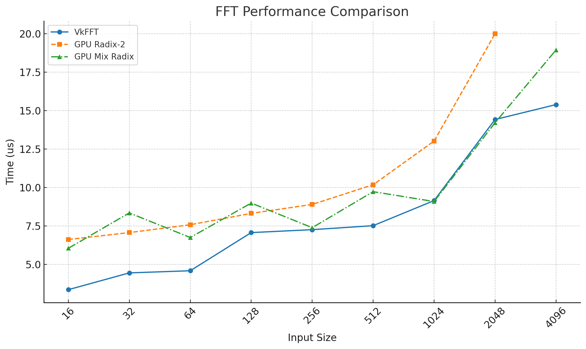
Through this work, I applied the knowledge gained from the Parallel Programming course to this project, achieving comparable results in specific cases to one of the most optimized GPU FFT libraries.
This project also highlighted that there is still much for me to explore to fully uncover the potential of GPUs.
For instance, sizes larger than 4096 are worth further investigation, where optimizing global memory access patterns becomes increasingly critical.